The teapot in a city: a paradigm shift in urban climate modeling Abstract and accompanying material

Corresponding authors: N. Villefranque (najda.villefranque@lmd.ipsl.fr) and F. Hourdin (hourdin@lmd.ipsl.fr)

The article

Urban areas are a high-stake target of climate change mitigation and adaptation measures. To understand, predict and improve the energy performance of cities, the scientific community develops numerical models that describe how they interact with the atmosphere through heat and moisture exchanges at all scales. In this review, we present recent advances that are at the origin of last decade's revolution in computer graphics, and recent breakthroughs in statistical physics that extend well established path-integral formulations to non-linear coupled models. We argue that this rare conjunction of scientific advances in mathematics, physics, computer and engineering sciences opens promising avenues for urban climate modeling and illustrate this with coupled heat transfer simulations in complex urban geometries under complex atmospheric conditions. We highlight the potential of these approaches beyond urban climate modeling, for the necessary appropriation of the issues at the heart of the energy transition by societies.

The film

This film was rendererd using physically-based rendering software htrdr. It demonstrates the capacity of Monte Carlo path-tracing methods to handle large scale ratios from large cloud fields to cities to buildings to trees and down to a teapot.

The figures

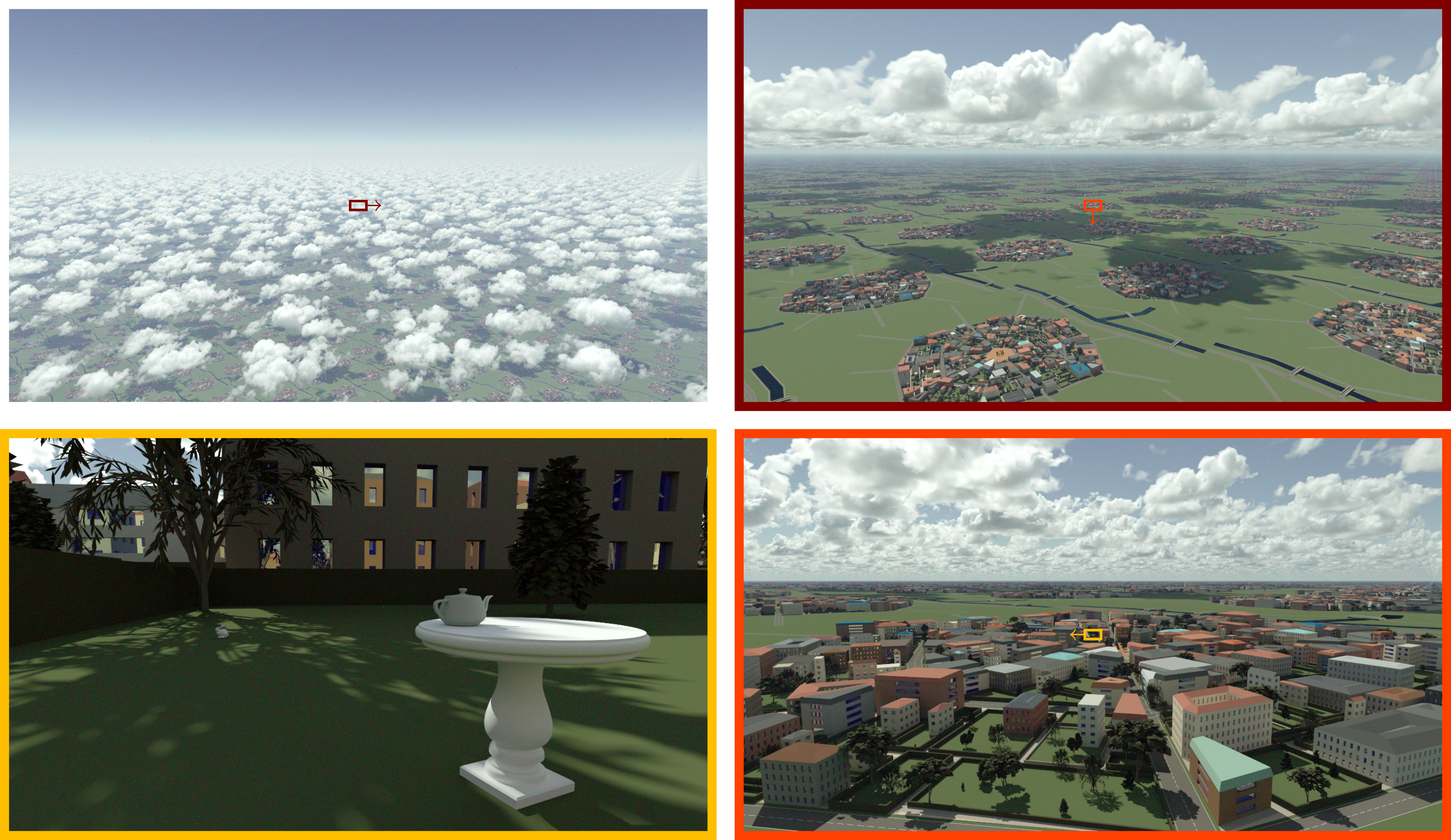
Figure 1. The teapot in a city under cumulus clouds, in reference to the ``teapot in the stadium" problem. The four pictures are sampled from an animated movie we produced using the htrdr model (35) that solves radiative transfer in the atmosphere and in cities. Each image features a different cloud field, camera and sun positions. Periodic conditions were used for the city geometry and the cloud fields to demonstrate insensitivity to the scene dimension. Cities and cloud fields of larger extent can be rendered with open boundary conditions as easily, provided that the data is available. The urban geometry was generated using procedural generator based on sampling distributions that represent the buildings characteristics (height, spacing...) and various tree geometries. The spectrally varying radiative properties of the materials were taken from the Spectral Library of Impervious Urban Materials (SLUM) database (36). The cloudy atmosphere was simulated using the Meso-NH Large-Eddy Simulation (LES) model (31, 37) and represents a typical fair-weather cumulus field evolving over a flat ground (38) at 8 meter resolution on a 15 x 15 x 4 km3 domain with horizontally periodic boundary conditions with 3D fields output every 15 seconds between 11:30 and 13:00 Local Solar Time (LST).

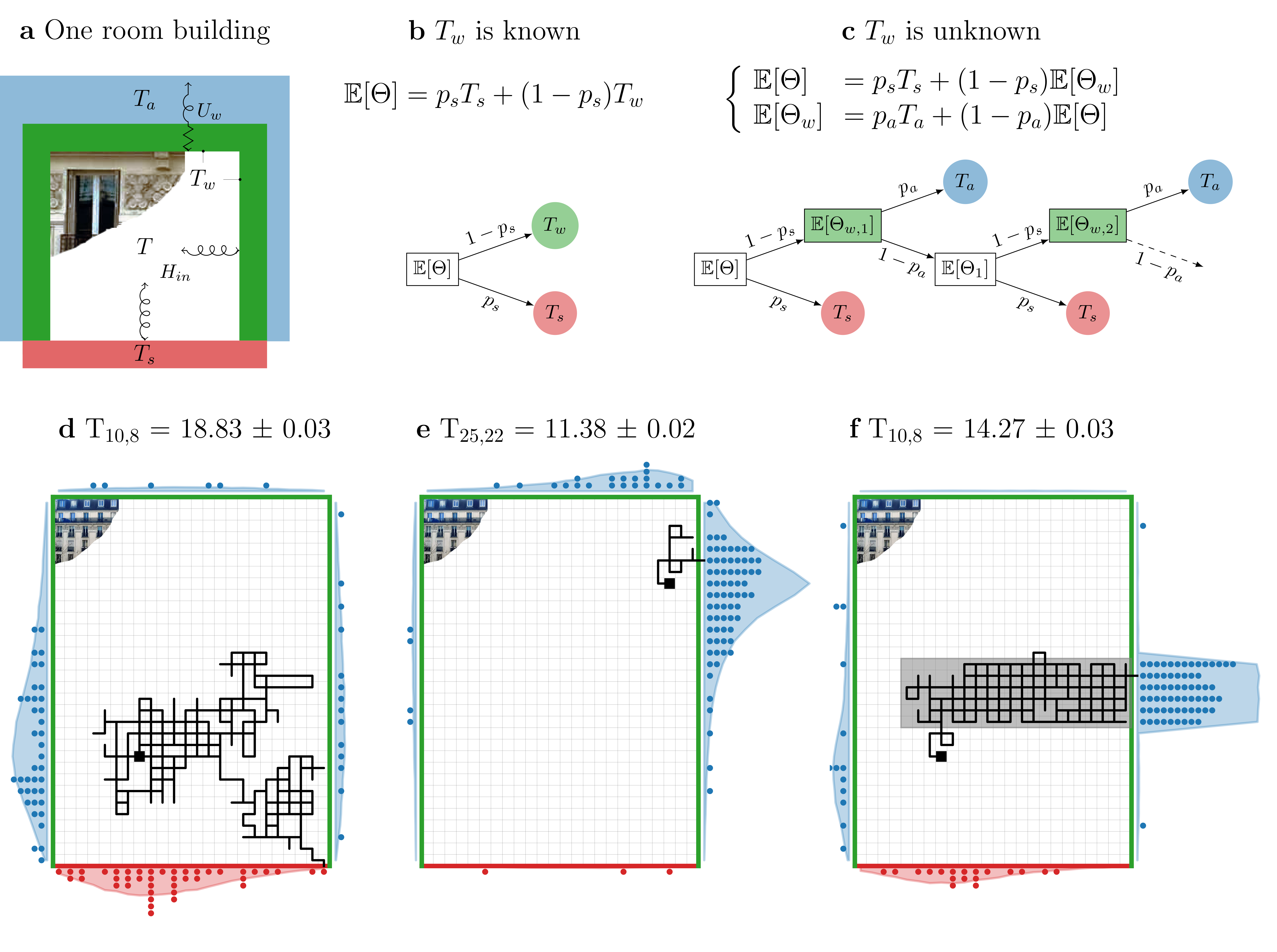
Figure 2. Heat transfers in 2D buildings of a-c one room and d-f N x M rooms. a, T is the temperature of the room's perfectly-mixed air, Ts the temperature of the ground floor, Tw the temperature of the three other walls, Ta is the temperature of the environmental perfectly-mixed air. Heat exchange between the inside air and the interior walls is driven by convection, with convective thermal conductance (CTC) Hin. Heat exchange between the interior walls and the outside air is driven by conduction in the wall and convection outside, of global thermal conductance Uw. b, T is the average of Tw and Ts, which is also the expectation of Theta whose outcomes are Ts with probability ps and Tw with probability 1-ps. c, Tw is itself the expectation of Thetaw. One realization of Theta is sampled by first sampling Thetaw,n and then Thetan successively until an outcome (Ts or Ta) is found. (Thetaw,n)n=1,..N and (Thetan)n=1,..N are collections of independent and identically distributed random variables that have the same probability law as Thetaw and Theta respectively. d-f, Ti,j is the temperature in room (i, j) (black square). The exterior walls have the same properties as in a, Ta = 10°C, Ts = 30°C. The interior walls all have the same CTCs except in the gray zone of g where they are a hundred times larger, which is symptomatic of a thermal bridge. The first sampled path (black line), the end locations of the first 100 sampled paths (blue and red points) and the distribution of the end locations of the 100,000 sampled paths (blue and red shadings) are shown for each simulation. The building heat flux is estimated by computing the average temperature of the outer rooms for e and g, as well as for a setup similar to e but with twice as many storeys in the building (the building is twice as high).

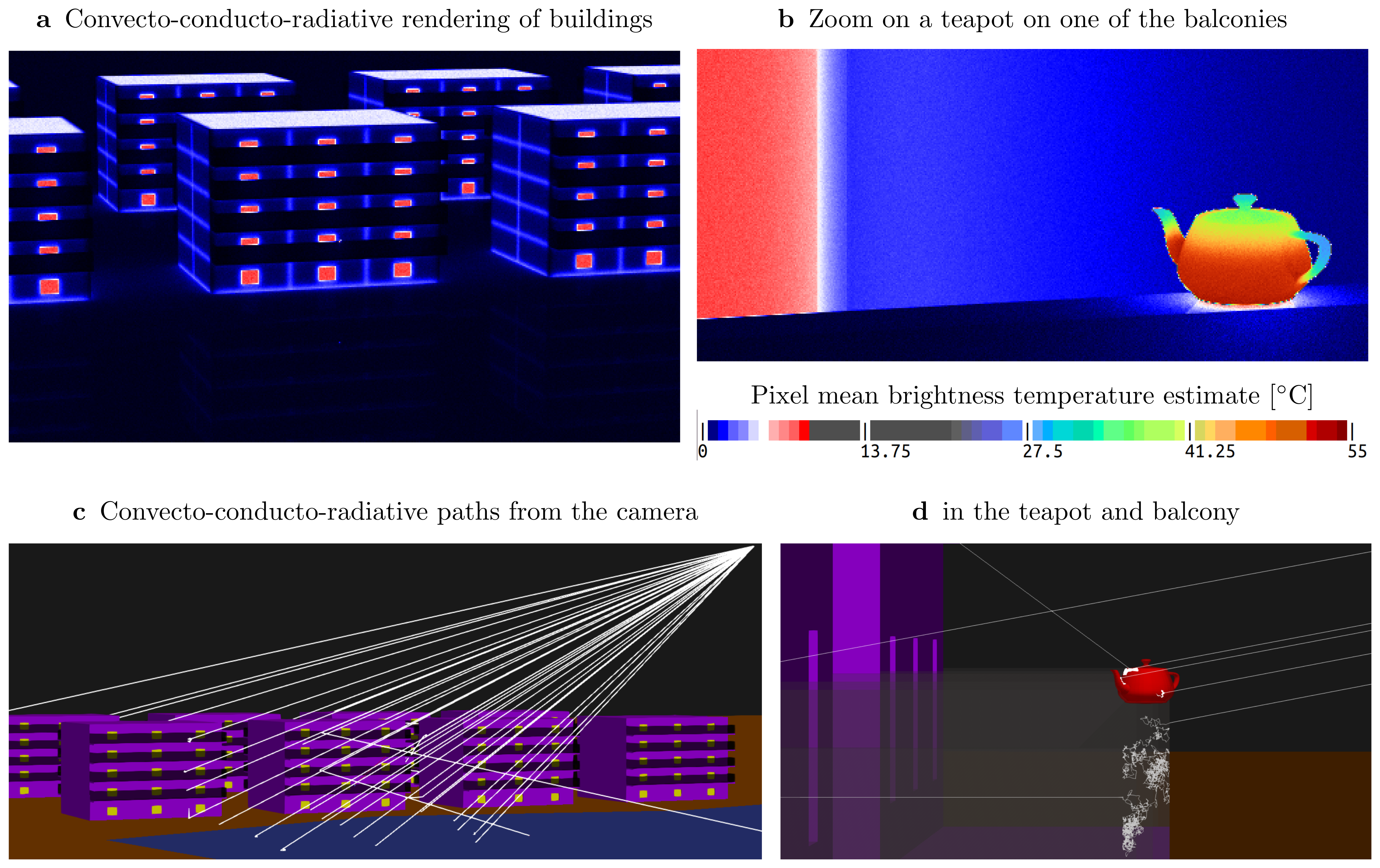
Figure 3. Physical infrared rendering of 3D buildings near a lake, in steady state, at night. The brightness temperature equivalent to the radiation emitted by the buildings, ground and atmo- sphere and received at the virtual camera is computed in each pixel by solving detailed heat transfers in the scene, using the Stardis software (http://meso-star.com/projects/ stardis/stardis.html). Paths start at the camera; conduction is simulated using δ- sphere walks inside the solids radiative exchanges are sampled between surfaces. Paths stop upon reaching a boundary condition: the temperature of the atmosphere (0°C), and rooms (20°C) by convection or the brightness temperature of the atmosphere (0°C) by radiation. They can also stop in the teapot which contains water at an imposed temperature of 60°C. a,b, results of convective-conductive-radiative Monte Carlo simulations for two views: a, a few buildings and b, a zoom on the teapot. Note that in a, the teapot is already on the first floor balcony of the middle building; it increases the mean brightness temperature of one of the pixels inside the red frame. c,d, 3D visualization of the scene and of a few paths sampled during the simula- tions. The scene consists of 33,958 facets (10,234 facets to describe the teapot and 23,724 for the buildings). Each image consists of 480x280 independent Monte Carlo estimates (one per pixel, 512 paths each)

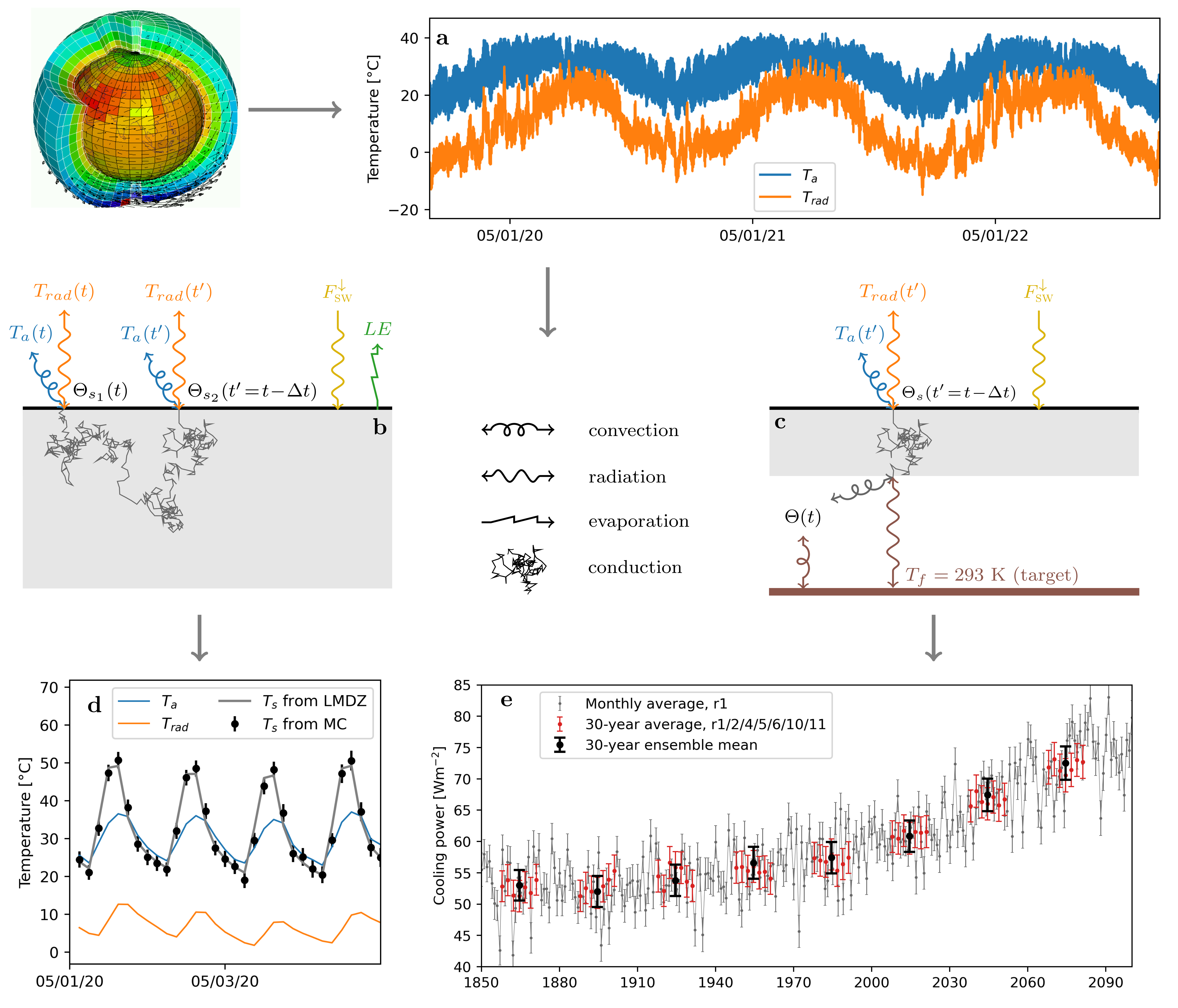
Figure 4. Time-varying meteorological conditions are used as inputs and parameters in path- integral heat transfer models. a, the air temperature at 2 meters above the surface (Ta) and the atmospheric brightness temperature (Trad) issued from a climate change simulation performed with the IPSL-CM6A-LR global model (74), available at a 3 hour frequency over 250 years. The variables retrieved from the climate archive are: Ta; the downwelling longwave (FdownLW , used to compute Trad) and swortwave (FdownSW) radiative fluxes at the surface; the sensible (H) and latent (LE) turbulent heat fluxes; and the surface temperature Ts. H and Ts are used to compute a convective exchange coefficient h = H/(Ts - Ta). LE and FdownSW are imposed fluxes. The data correspond to a gridpoint in Sahel. b-c, Random path representation of the heat transfer models used to estimate: d, the surface temperature of a homogeneous soil of thermal inertia 1500 J m^-2 s^-1/2 K, and e, the air-conditioning power to maintain a simplified room's floor at 293 K. d, instantaneous temperatures every 3 h during four days: Monte Carlo estimates of Ts (black dots) and Ts, Ta and Trad from the climate archive (gray, blue and orange lines). e, May averages of air-conditioning power from 1850 to 2100: every year (gray dots); averaged over 30 years (red dots), each red dot corresponds to a different member of an ensemble simulation (75); averaged over 30 years and over the ensemble members (black dots). Dots and error bars in d and e correspond to Monte Carlo estimates based on 30k paths and their associated 99.7% confidence interval.

The models scientific basis

The codes

htrdr will let you compute images of cloud fields as displayed in Fig. 1. The data representing the cloud fields that were used in Fig. 1 are too heavy to be shared through this webpage but they are available on demand. They were obtained by high-resolution simulations using the French atmospheric model Meso-NH. Other lighter cloud fields are provided, along with several ground geometries including the city, in the htrdr starter pack.

This archive contains the python code that will let your reproduce Fig. 2 of the main manuscript as well as Figs SI2, SI3, SI4.

stardis will let you compute images of buildings as displayed in Fig. 3. The building geometry, along with several others, is provided in the stardis starter pack.

This archive contains the data and python scripts that will let your reproduce Fig. 4 of the main manuscript as well as Figs SI5, SI6, SI7. The data was produced using Fortran and bash code that can be downloaded here.